A solar cellular automata model
issued from reduced MHD
E. Buchlin † , V. Aletti , S. Galtier , M. Velli† and J.-C. Vial
†
I.A.S., CNRS – Université Paris-Sud, bât. 121, 91405 Orsay Cedex, France
Dipartimento di Astronomia e Scienza dello Spazio, Università di Firenze, 50125 Firenze, Italy
Istituto Nazionale Fisica della Materia, Sezione A, Università di Pisa, 56100 Pisa, Italy
Abstract. A three-dimensional cellular automata (CA) model inspired by the reduced magnetohydrodynamic equations is
presented to describe impulsive events generated along a coronal magnetic loop. It consists of a set of planes, distributed
along the loop, between which the information propagates through Alfvén waves. Statistical properties in terms of power laws
are obtained in agreement with SoHO observations of X-ray bright points of the quiet Sun. Physical meaning and limits of the
model are discussed.
INTRODUCTION
It is now commonly accepted that the ultimate source
of energy for coronal heating lies in the photosphere,
and that the questions to address are the transfer, the
storage, and the release of this energy. These processes
involve MHD and structures extending over a large range
of scales. This is consistent with observational statistics
of impulsive events, whose luminosity, peak luminosity
and duration distributions are power-laws (Dennis 1985
[1], Crosby et al. 1993 [2]).
This CA model attempts to describe the statistics of
such events. It represents a coronal loop whose footpoints are anchored in the photosphere and are randomly
moved.
x
B
B0
L
y
z
FIGURE 1. Coronal loop above the photosphere (top) and
correspondence with the geometry of the loop model (bottom).
DESCRIPTION OF THE MODEL
In our CA model, a 3D regular grid is made up of a set
of planes distributed along the loop and orthogonal to its
axis, as shown on Fig. 1. Both boundary planes represent the photospheric footpoints, while the intermediate
planes represent the loop itself, as if it were unbent.
The presence of a strong axial magnetic field in the
loop leads to essentially 2D dynamics, i.e. perpendicular to the mean magnetic field. A quite good model in
this case is given by the reduced magnetohydrodynamics
(RMHD) equations, which describe the evolution of the
magnetic and velocity fields, and include Alfvén wave
propagation, energy dissipation and non-linear dynamics:
∂t v
v
∇
v
∂t b
v
∇
b
b0 ∂z b
ν∆ v
b ∇ b ∇b2 2
b0 ∂z v
η∆ b
b ∇ v
The non-linear dynamics are modeled through an onoff mechanism, triggered by a dissipation criterion. For
our model, we choose this dissipation criterion to be a
current density threshold.
Energy is input as random magnetic and velocity fields
on both photospheric planes, with a 2D spatial powerlaw spectrum of index α , and it is transported by Alfvén
waves to all loop planes. As a result, energy grows until
CP679, Solar Wind Ten: Proceedings of the Tenth International Solar Wind Conference,
edited by M. Velli, R. Bruno, and F. Malara
© 2003 American Institute of Physics 0-7354-0148-9/03/$20.00
335
a quasi-stationary state is obtained, when dissipation is
sufficient to compensate for the energy input.
RESULTS
Dissipations. Energies of dissipations span a wide
range of values (four orders of magnitude). They grow
until the quasi-stationary phase is reached, as indicated
on Fig. 2 (c) and (d).
FIGURE 3. Example of histogram of magnetic energy dissipation dEi in a plane i of the simulation box.
FIGURE 4. Example of histogram of magnetic energy dissipation dE ∑ dEi in the whole simulation box.
FIGURE 2.
log) and dE
Time series of energy dissipations Ei (a: lin; b:
∑ dEi (c: lin; d: log).
Energy histograms power-laws. Histograms of elementary energy dissipations dE i in a plane i fit to powerlaws over 2 to 3 decades, as seen on Fig. 3. The indices ζ
of these power-law depend on the parameters, and their
absolute values are between 1 and 2. However, powerlaws of histograms of energies dissipated in the whole
simulation box (i.e. seen at a lower spatial resolution) are
narrower and present steeper slopes (Fig. 4).
The signal dEi t “seems intermittent” (Fig. 2) and its
histograms are consistent with what is expected. However, this is not sufficient: intermittence in MHD turbulence needs also to be characterized by wide wings of
PDFs at small scales, or, equivalently, some properties of
structure functions or flatness.
Location of dissipations. Dissipations do not mainly
occur in current sheets, and these structures are not predominant structures as in MHD simulations (see Fig. 5).
This is a limit due to the dissipation criterion chosen to
model the non-linear dynamics: it is indeed well established that the terms of the (R)MHD equations which
336
lead to structures like current sheets, where reconnection
occurs, are the non-linear terms.
It could be interesting to use a more realistic dissipation criterion. However, a CA model is only supposed to
produce realistic statistics, not realistic fields.
60
60
50
50
40
40
30
30
20
20
10
10
0
0
0
10
20
30
40
50
60
0
10
20
30
40
50
60
FIGURE 5. Two examples of magnetic field (lines) and current density (background) in a plane.
Durations of events. Durations of elementary events
extend over two decades. Histograms can be obtained,
but these two decades of duration span are not enough to
perform relevant power-law fitting (Fig. 6).
The duration of events is correlated with their energy,
like dEi ∝ dti1 75 (Fig. 7), in agreement with observations
(see discussion). This correlation can also be seen by
plotting event energy histograms for different ranges of
event durations, as on Fig. 8.
Parametric study. An extensive parametric study
was performed, with at least 200 000 time steps computed for more than 20 parameters sets. It shows the
variability of the event energy histogram slope ζ as a
function of the loading index α (Fig. 9). For low α ’s,
the characteristic power-law shape of histograms is more
difficult to obtain, thus the ζ ’s are perhaps not very relevant power-law indices. On the contrary, for high α ’s, the
power-laws are wide and robust, and ζ 16, appears
to be a “universal” power-law index for the histograms of
dEi . This “universal” behavior is similar to the behavior
of SOC (self-organized criticality) systems, from basic
sandpile models (Bak et al. 1988 [3]) to more elaborate
solar-like SOC models like Vlahos et al. 1995 [4] or Isliker et al. 2000 [5].
Changing the other parameters (resistivity, dissipation
efficiency) does not really affect the histograms, confirming the “universal” behavior of the slope.
FIGURE 6. Typical histogram of events durations in a plane
of the simulation box.
FIGURE 9. Variability of event energy histogram slope ζ vs. loading spectrum index α .
FIGURE 7.
Correlation between events duration and energy.
DISCUSSION
Comparison with observations
FIGURE 8. Events durations separate populations, from low
duration (left, dashed) to long duration (right, dashed), which
have different energy distributions. The solid line is the sum of
other histograms; it is the same curve as in Fig. 3.
337
Statistical observations of bright points luminosities
lead to power-law histograms of index 16 to 26.
When taking into account an observational bias due to
temperature, Aschwanden and Charbonneau [6] show
that these observations lead to a ”universal” index which
could be even less steep than 16. These values are
compatible with the power-law slopes of event energy
distributions produced by our model.
Furthermore, the existence of such a bias emphasizes
the importance for new models to produce observables,
i.e. variables whose statistics can be directly compared
to the statistics of observational data. An event energy is
indeed not the same variable as an event luminosity and
could have different statistics.
We also pointed out in Fig. 3 and 4 a possible effect of
spatial resolution on the statistics, which is discussed on
SoHO/EIT observational data in Aletti et al. [7]. Indeed,
the interpretation of several subresolution events in a
single pixel as one single event, which is unavoidable
when analyzing observations, changes the slope and the
shape of histograms compared to histograms of really
elementary events.
At last, observations from Berghmans et al. [8] show
that event durations scale like their radiative loss at the
power 05, which is in quite good agreement with our
prediction 1176 057 (see Fig. 7).
Conclusion
This CA model, which tries to stay close enough to the
MHD equations and to the physics of coronal magnetic
loops, succeeds in reproducing some of the characteristics of the statistics of events observed on the Sun. However, progress still remains to be done to model more
accurately the non-linear terms of the MHD equations
leading to the magnetic reconnection process, either by a
better dissipation criterion in the frame of threshold dynamics, or even better, by incorporating these non-linear
terms in a more realistic way in the dynamics of a new
model. More accurate event distribution power-law indices could then be compared to Hudson’s [9] critical
index of -2 and thus give a clue about Parker’s hypothesis of nanoflares; these works could help interpreting the
statistical observations of flares.
ACKNOWLEDGMENTS
The authors acknowledge partial financial support from
PNST (Programme National Soleil–Terre). E. Buchlin
thanks the Scuola Normale Superiore of Pisa for support
and accommodation.
338
REFERENCES
1. Dennis, B. R., Sol. Phys., 100, 465–490 (1985).
2. Crosby, N. B., Aschwanden, M. J., and Dennis, B. R., Sol.
Phys., 143, 275–299 (1993).
3. Bak, P., Tang, C., and Wiesenfeld, K., Phys. Rev. A, 38,
364–374 (1988).
4. Vlahos, L., Georgoulis, M., Kluiving, R., and Paschos, P.,
Astron. Astrophys., 299, 897+ (1995).
5. Isliker, H., Anastasiadis, A., and Vlahos, L., Astron.
Astrophys., 363, 1134–1144 (2000).
6. Aschwanden, M. J., and Charbonneau, P., ApJ, 566,
L59–L62 (2002).
7. Aletti, V., Velli, M., Bocchialini, K., Einaudi, G.,
Georgoulis, M., and Vial, J.-C., ApJ, 544, 550–557
(2000).
8. Berghmans, D., Clette, F., and Moses, D., Astron.
Astrophys., 336, 1039–1055 (1998).
9. Hudson, H. S., Sol. Phys., 133, 357–369 (1991).
© Copyright 2026 Paperzz